Turbulent fluid flows in pipes and open channels play an important role in hydraulics, chemical engineering, transportation of hydrocarbon, air duct design, etc.
1
These flows induce a significant loss of energy depending on the flow regime and the friction on the rigid boundaries. When fluid flows through a pipe, friction between the pipe wall and the fluid works against the flow and is one of the most important parameters in determining a pipeline's capacity
2
The head loss (hf) due to friction undergone by a fluid motion in a pipe is usually calculated through the Darcy-Weisbach relation.
hloss = f (L/D) u2/2g
Where f = friction factor or friction coefficient.
The term u2/2g is known as "Velocity Head" where
u = flow velocity and
g = acceleration of gravity.
L= length of duct/pipe
D is hydraulic diameter of the duct.
3
The friction factor (f ) is a measure of the shear stress (or shear force per unit area) that the turbulent flow exerts on the wall of a pipe and expressed in dimensionless form as f = τ/ρū2, where, τ is the shear stress, ρ is the density of the liquid that flows in the pipe and ū the mean velocity of the flow.
4
For laminar flow (Reynolds number, R ≤ 2100), the friction factor is linearly dependent on R, and calculated from the well-known Hagen-Poiseuille equation:
λ = 64 /R
Where, R, the Reynolds number, is defined as ū D/ ν where ν is the kinematic viscosity = m/r, the ratio of viscosity and density.
Flow in offshore gas pipelines is characterized by high Reynolds numbers, typically highest, in the order of 107, due to the low viscosity and the relative high density of natural gas at typical operating pressures (100-180 bar). For normal liquid lines, the Reynolds number is normally in the range of 5x10⁴ to 1x10⁶
5
In turbulent flow (R≥ 4000), the friction factor, f depends upon the Reynolds number (R) and on the relative roughness of the pipe, e/D, where, e is the average roughness height of the pipe
6
When k is very small compared to the pipe diameter D i.e. e/D→0, and f depends only on R.
7
SMOOTH LAMINAR FLOW REGIME: When k/D is of a significant value, at low R, the flow can be considered as in smooth regime (there is no effect of roughness). In a smooth pipe flow, the viscous sub layer completely submerges the effect of e
on the flow. In this case, the friction factor f is a function of R and is independent of the effect of e on the flow.
8
CRITICAL ZONE: Fluids with a Reynolds number between 2000 and 4000 are considered unstable and can exhibit either laminar or turbulent behavior. This region is commonly referred to as the critical zone and the friction factor can be difficult to accurately predict. Judgment should be used if accurate predictions of fluid loss are required in this region. Colebrook equation can be examined to get a rough estimate of friction in this region.
9
If the Reynolds number is beyond 4000, the fluid is considered turbulent and the friction factor is dependent on the Reynolds number and relative roughness
TRANSITION REGIME: As R increases, the flow becomes transitionally rough, called as transition regime in which the friction factor rises above the smooth value and is a function of both k and R.
ROUGH TURBULENT REGIME: As R increases more and more, the flow eventually reaches a fully rough regime in which f is independent of R.
In this zones the friction factor f is calculated by Colebrook’s equation (Colebrook 1938-39)
10
Nikuradse (1933) verified the Prandtl’s mixing length theory and proposed the following universal resistance equation for fully developed turbulent flow in smooth pipe;
1/= 2 log (R ) - 0.8
11
In case of rough pipe flow, the viscous sub layer thickness is very small when compared to roughness height and thus the flow is dominated by the roughness of the pipe wall and f is the function only of k/D and is independent of R. The following form of the equation is first derived by Von Karman (Schlichting, 1979) and later supported by Nikuradse’s experiments
1/= 2 log (D/e ) + 1.74
12
COLEBROOK EQUATION: The Colebrook–White equation estimates the (dimensionless) Darcy–Weisbach friction factor f for fluid flows in filled pipes. For transition regime of flow, in which the friction factor varies with both R and e/D, the equation universally adopted is due to Colebrook and White (1937) proposed the following equation

e is relative roughness
f is the friction factor
Re is Reynolds numbers.
The Colebrook equation can be used to calculate the friction coefficients in different kinds of fluid flows - air ventilation ducts, pipes and tubes with water or oil, compressed air and much more.
13
Colebrook Equation covers not only the transition region but also the fully developed smooth and rough pipes. By putting e → 0, this reduces to equation for smooth pipes and as R→∞, it forms equation for rough pipes.
Colebrook’s transition curve merges asymptotically into the curves representing laminar and completely turbulent flow.
14
In a smooth pipe flow, the viscous sub layer completely submerges the effect of k on the flow. In this case, the friction factor f is a function of R and is independent of the effect of k on the flow.
15
In case of rough pipe flow, the viscous sub layer thickness is very small when compared to roughness height and thus the flow is dominated by the roughness of the pipe wall and f is the function only of k/D and is independent of R.
16
The Colebrook equation has two terms. The first term, (e/D)/3.7, is dominant for gas flow where the Re is high. The second term, 2.51/Re, is dominant for fluid flow where the relative roughness lines converge (smooth pipes).
17
Moody (1944) presented a friction diagram for commercial pipe friction factors based on the Colebrook–White equation, which has been extensively used for practical applications. This is known as Moody's Chart or Diagram.
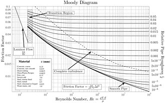
In the “Complete Turbulence” region, these lines are “flat”, meaning that they are independent of the Reynolds Number. In the “transition Zone”, the lines are dependent on Re and . When the lines converge in the “smooth zone” the fluid is independent of relative roughness.
Recently it has come to know that Moody diagram is only +/-15% accurate. Glenn O. Brown (professor, Oklahoma State University, OK) recently in his published on internet wondered why, for more than 6 decades, the Moody diagram was used unmodified and still in use same way.
18
The traditional Moody diagram is still a much widely used method to determine f, even though some major limitations apply to it: It over-estimates the ‘smooth pipe’-friction for Re > 106, and it is very inaccurate around Re = 104
19
Because of Moody’s work and the demonstrated applicability of Colebrook-White equation over a wide range of Reynolds numbers and relative roughness value e/D, COLEBROOK equation has become the universally accepted standard for calculating the friction factors for rough pipes.
20
Since the mid-1970s, many alternative explicit equations have been developed to avoid the iterative process that is inherent in Colebrook- White equation. These equations give a reasonable approximation; however, they tend to be less universally accepted.
21
One of the major draw back of Colebrook equation is that it is implicit! However, implicit equations can be solved in Excel, which has been discussed in this book in great detail.
22
Some researchers have found that the Colebrook–White equation is inadequate for pipes smaller than 2.5 mm
Zagarola (1996) has indicated that the Prandtl’s law of flow in smooth pipes was not accurate for high Reynolds numbers and the Colebrook-White correlation (which was based on the Prandtl’s law of flow) is not accurate at high Reynolds numbers1.
22
The major cost of piping and pumping system is always thought to be the capital investment on the piping and pumping units. However, the recurrence expenditure on the power consumption has to be given due consideration because generally the recurrence expenditure over the years far outweigh the capital investment. Hence the major length of the pipeline is designed with a view to minimize both the power requirement and pipe material simultaneously2.
23
Idelchik summarizes roughness factors for 80 materials including metal tubes, conduits made from concrete and cement; and wood, plywood, and glass tubes.
Idelchik, I.E., M.O. Steinberg, G.R. Malyavskaya, and O.G. Martynenko.
1994. Handbook of hydraulic resistance, 3rd ed. CRC Press
24
Typical values of absolute roughness are 0.0015 mm for PVC, drawn tubing, glass and 0.045 mm for commercial steel/welded steel and wrought iron
25
Fast, accurate and robust resolution of the Colebrook equation is necessary to design computations and flow simulations. A fast and simple computational method to find out solution for Colebrook as presented in this book, is expected to effectively contribute to such optimizations.
26
Notwithstanding certain shortcomings as reported by certain researchers, the Colebrook equation is currently the most accepted equation for calculating the friction factors in most of the industrial flow calculations.
1 Zagarola, M. V., ‘‘Mean-flow Scaling of Turbulent Pipe Flow,’’ Ph.D.thesis, Princeton University, USA, 1996.
2 “Energy Efficient Pipe Sizing and Piping Optimization”– A book by the same author. Visit www.ColebrookEquation.com for more details

THE ABOVE MATERIAL IS PUBLISHED HERE FROM THE BELOW BOOK WITH PERMISSION OF THE AUTHOR
